Quick Start Guide
In Aboleth we use function composition to compose machine learning models.
These models are callable python classes that when called return a TensorFlow
computational graph (really a tf.Tensor). We can best demonstrate this with
a few examples.
Logistic Classification
For our first example, lets make a simple logistic classifier with \(L_2\) regularisation on the model weights:
import tensorflow as tf
import aboleth as ab

layers = (
    ab.InputLayer(name="X") >>
    ab.Dense(output_dim=1, l1_reg=0, l2_reg=.05) >>
    ab.Activation(tf.nn.sigmoid)
)
Here the right shift operator, >>, implements functions composition (or
specifically, a writer monad) from the innermost function to the outermost.
The above code block has has implemented the following function,
where \(\mathbf{w} \in \mathbb{R}^D\) are the model weights,
\(\mathbf{y} \in \mathbb{N}^N_2\) are the binary labels, \(\mathbf{X}
\in \mathbb{R}^{N \times D}\) are the predictive inputs and
\(\sigma(\cdot)\) is a logistic sigmoid function. At this stage layers
is a callable class (ab.baselayers.MultiLayerComposite), and no
computational graph has been built. ab.InputLayer allows us to name our
inputs so we can refer to them later when we call our class layers. This is
useful when we have multiple inputs into our model, for examples, if we want to
deal with continuous and categorical features separately (see Multiple Input Data).
So now we have defined the structure of the predictive model, if we wish we can create its computational graph,
net, reg = layers(X=X_)
where the keyword argument X was defined in the InputLayer and X_
is a placeholder (tf.placeholder) or the actual predictive data we want to
build into our model. net is the resulting computational graph of our
predictive model/network, and reg are the regularisation terms associated
with the model parameters (layer weights in this case).
If we wanted, we could evaluate net right now in a TensorFlow session,
however none of the weights have been fit to the data. In order to fit the
weights, we need to define a loss function. For this we need to define a
likelihood model for our classifier, here we choose a Bernoulli distribution
for our binary classifier (which corresponds to a log-loss):
likelihood = tf.distributions.Bernoulli(probs=net)
log_like = likelihood.log_prob(Y_)
which returns a tensor that implements the log of a Bernoulli probability mass function,
This is an integral part of our loss function. Here we have used \(p_n\) as shorthand for \(p(y_n = 1)\).
Note
We actually find it is more numerically stable to define Bernoulli likelihoods with logits:
likelihood = tf.distributions.Bernoulli(logits=net)
Where:
layers = (
    ab.InputLayer(name="X") >>
    ab.Dense(output_dim=1, l1_reg=0, l2_reg=.05) >>
)
net, reg = layers(X=X_)
The Bernoulli class then computes the sigmoid activation internally.
Now we have enough to build the loss function we will use to optimize the model weights:
loss = ab.max_posterior(log_like, reg)
This is a maximum a-posteriori loss function, which can be thought of as a
maximum likelihood objective with a penalty on the magnitude of the weights
from a Gaussian prior (controlled by l2_reg or \(\lambda\)),
Now we have enough to use the tf.train module to learn the weights of our
model:
optimizer = tf.train.AdamOptimizer()
train = optimizer.minimize(loss)

with tf.Session() as sess:
    tf.global_variables_initializer().run()

    for _ in range(1000):
        sess.run(train, feed_dict={X_: X, Y_: Y})
This will run 1000 iterations of stochastic gradient optimization (using the
Adam learning rate algorithm) where the model sees all of the data every
iteration. We can also run this on mini-batches, see ab.batch for a simple
batch generator, or TensorFlow’s train and data modules for a more
comprehensive set of utilities (we recommend looking at
tf.train.MonitoredTrainingSession,
and tf.data.Dataset)
Now that we have learned our classifier’s weights, \(\hat{\mathbf{w}}\), we will probably want to use for predicting class label probabilities on unseen data \(\mathbf{x}^*\),
This can be very easily achieved by just evaluating our model on the unseen predictive data (still in the TensorFlow session from above):
probs = net.eval(feed_dict={X_: X_query})
However, you may find that probs.shape will be something like (1, N, 1)
where N = len(X_query). Aboleth made a new, 0th, axis here, and we’ll talk
about why this is the case in the next section.
Note
If you used logits as per the above note, then the prediction becomes:
probs = likelihood.probs.eval(feed_dict={X_: X_query})
And that is it!
Bayesian Logistic Classification
Aboleth is all about Bayesian inference, so now we’ll demonstrate how to make a variational inference version of the logistic classifier. Now we explicitly place a prior distribution on the weights,
Here \(\psi\) is the prior weight standard deviation (note that this corresponds to \(\sqrt{\lambda^{-1}}\) in the MAP logistic classifier). We use the same likelihood model as before,
and ideally we would like to infer the posterior distribution over these weights using Bayes’ rule (as opposed to just the MAP value, \(\hat{\mathbf{w}}\)),
Unfortunately the integral in the denominator is intractable for this model. This is where variational inference comes to the rescue by approximating the posterior with a known form – in this case a Gaussian,
where \(\boldsymbol{\mu} \in \mathbb{R}^D\) and \(\boldsymbol{\Sigma} \in \mathbb{R}^{D \times D}\). To make this approximation as close as possible, variational inference optimizes the Kullback Leibler divergence between this and true posterior using the evidence lower bound, ELBO, and the reparameterization trick in [1]:
One question you may ask is why would we want to go to all this bother over the MAP approach? Specifically, why learn an extra \(\mathcal{O}(D^2)\) number of parameters over the MAP approach? Well, a few reasons, the first being that the weights are well regularised in this formulation, for instance we can actually learn \(\psi\), rather than having to set it (this optimization of the prior is called empirical Bayes). Secondly, we have a principled way of incorporating modelling uncertainty over the weights into our predictions,
This will have the effect of making our predictive probabilities closer to 0.5 when the model is uncertain. The MAP approach has no mechanism to achieve this since it only learns the mode of the posterior, \(\hat{\mathbf{w}}\), with no notion of variance.
So how do we implement this with Aboleth? Easy; we change layers to the
following,
import numpy as np
import tensorflow as tf
import aboleth as ab

n_samples_ = tf.placeholder_with_default(5, [])
layers = (
    ab.InputLayer(name="X", n_samples=n_samples_) >>
    ab.DenseVariational(output_dim=1, prior_std=1., full=True) >>
    ab.Activation(tf.nn.sigmoid)
)
Note we are using DenseVariational instead of Dense. In the
DenseVariational layer the full parameter tells the layer to use a full
covariance Gaussian, and prior_std is value of the weight prior standard
deviation, \(\psi\). Also we’ve set n_samples=5 (as a default value of
a place holder) in the InputLayer, this lets the subsequent layers know
that we are making a stochastic model, that is, whenever we call layers
we are actually expecting back 5 samples of the model output. This argument
defaults to 1, which is why we got a one-dimensional 0th axis in the last
section. In this instance a setting of 5 makes the DenseVariational layer
multiply its input with 5 samples of the weights from the approximate
posterior, \(\mathbf{X}\mathbf{w}^{(s)}\), where \(\mathbf{w}^{(s)}
\sim q(\mathbf{w}),~\text{for}~s = \{1 \ldots 5\}\). These 5 samples are then
passed to the Activation layer. We have used a place holder here because we
usually want to use more samples of the network for prediction than for
training.
Then like before to complete the model specification:
net, kl = layers(X=X_)
likelihood = tf.distributions.Bernoulli(probs=net)
log_like = likelihood.log_prob(Y_)
loss = ab.elbo(log_like, KL=kl, N=10000)
The main differences here are that reg is now kl, and we use the
elbo loss function. For all intents and purposes kl is still a
regularizer on the weights (it is the Kullback Leibler divergence between the
posterior and the prior distributions on the weights), and elbo is the
evidence lower bound objective. Here N is the (expected) size of the
dataset, we need to know this term in order to properly calculate the evidence
lower bound when using mini-batches of data.
We train this model in exactly the same way as the logistic classifier, however prediction is slightly different - that is we need to average the samples drawn from the network to get a predicted probability (as in the sum over weight samples above),
predict_p = tf.reduce_mean(net, axis=0)
probs = net.eval(predict_p,
                 feed_dict={X_: X_query, n_samples_: 20})
So probs also has a shape of \((N^*, 1)\), and we have used 20 samples to calculate the average probability.
Note
If you used logits in the likelihood, then the prediction becomes:
predict_p = tf.reduce_mean(likelihood.probs, axis=0)
probs = net.eval(predict_p,
                 feed_dict={X_: X_query, n_samples_: 20})
Approximate Gaussian Processes
Aboleth also provides the building blocks to easily create scalable (approximate) Gaussian processes. We’ll implement a simple Gaussian process regressor here, but for brevity, we’ll skip the introduction to Gaussian processes, and refer the interested reader to [2].
The approximation we have implemented in Aboleth is the random feature expansions (see [3] and [4]), where we can approximate a kernel function from a set of random basis functions,
with equality in the infinite limit. The trick is to find the right family of basis functions, \(\phi\), that corresponds to a particular family of kernel functions, e.g. radial basis, Matern, etc. This insight allows us to approximate a Gaussian process regressor with a Bayesian linear regressor using these random basis functions, \(\phi^{(s)}(\mathbf{X})\)!
We can easily do this using Aboleth, for example, with a radial basis kernel,
import tensorflow as tf
import aboleth as ab

lenscale = tf.Variable(1.)  # learn isotropic length scale
kern = ab.RBF(lenscale=ab.pos(lenscale))

n_samples_ = tf.placeholder_with_default(5, [])
layers = (
    ab.InputLayer(name="X", n_samples=n_samples_) >>
    ab.RandomFourier(n_features=100, kernel=kern) >>
    ab.DenseVariational(output_dim=1, full=True)
)
Here we have made lenscale a TensorFlow variable so it will be optimized,
and we have also used the ab.pos function to make sure it stays positive.
The ab.RandomFourier class implements random Fourier features [3], that
can model shift invariant kernel functions like radial basis, Matern, etc. See
ab.kernels for implemented kernels. We have also implemented random
arc-cosine kernels [4] see ab.RandomArcCosine in ab.layers.
Then to complete the formulation of the Gaussian process (likelihood and loss),
std = tf.Variable(1.)  # learn likelihood std. deviation

net, kl = layers(X=X_)
likelihood = tf.distributions.Normal(net, scale=ab.pos(std))
log_like = likelihood.log_prob(Y_)
loss = ab.elbo(log_like, kl, N=10000)
Here we just have a Normal likelihood since we are creating a model for
regression, and we can also get TensorFlow to optimise the likelihood standard
deviation, std.
Training and prediction work in exactly the same way as the Bayesian logistic classifier. Here is an example of the approximate GP in action (see Regression for a more detailed demonstration);
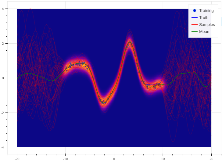
Example of an approximate Gaussian process with a radial basis kernel. We have shown 50 samples of the predicted latent functions, the mean of these draws, and the heatmap is the probability of observing a target under the predictive distribution, \(p(y^*|\mathbf{X}, \mathbf{y}, \mathbf{x}^*)\).
See Also
For more detailed demonstrations of the functionality within Aboleth, we recommend you check out the demos,
- Regression and SARCOS - for more regression applications.
- Multiple Input Data - models with multiple input data types.
- Bayesian Classification with Dropout - Bayesian nets using dropout.
- Imputation Layers - let Aboleth deal with missing data for you.
References
| [1] | Kingma, D. P. and Welling, M. Auto-encoding variational Bayes. In ICLR, 2014. |
| [2] | Rasmussen, C. E., and Williams, C. K. I. Gaussian processes for machine learning. Cambridge: MIT press, 2006. |
| [3] | (1, 2) Rahimi, A., & Recht, B. Random features for large-scale kernel machines. Advances in neural information processing systems. 2007. |
| [4] | (1, 2) Cutajar, K. Bonilla, E. Michiardi, P. Filippone, M. Random Feature Expansions for Deep Gaussian Processes. In ICML, 2017. |